
Introduction
This post is the third in a series - to get up to speed, have a read through the first post and the second post. In this series, I will show how I created the plots that Aiden published on Twitter here and here, alongside some commentary about the choices I made throughout the process and my own interpretations of the results.
Getting started
Load up the data and the libraries as we’ve done before.
library(readr)
library(knitr)
library(kableExtra)
library(ggplot2)
library(dplyr)

# Read the data into R
dataSource <- "https://raw.githubusercontent.com/jacquietran/soccerSalariesDataPublic/master/soccerSalariesDataPublic.csv"
soccerSalariesData <- read_delim(dataSource, delim = ",", col_names = TRUE, col_types = NULL)
Salaries by league and by discipline
Let’s compare how sport scientists and S&C coaches are paid in the different leagues.
# Subset of data frame to exclude dept == NA
soccerSalariesData3 <- soccerSalariesData %>%
    filter(!is.na(dept))
soccerSalariesData3$dept <- recode(
    soccerSalariesData3$dept,
    `Physical Performance` = "S&C")

# Set factor levels
soccerSalariesData3$dept <- factor(
    soccerSalariesData3$dept,
    levels = c("S&C", "Sport Science", "Both"))
soccerSalariesData3$leagueOfFirstTeam <- factor(
    soccerSalariesData3$leagueOfFirstTeam,
    levels = c(
        "Premier League", "Scottish Premiership", "Championship", "League 1", "League 2"))

# Create object to store axis labels with line breaks
labelsLeague <- c("PL", "SP", "C", "L1", "L2")

# Create a list to store common theme options for use across plots
plotFeatures <- theme(
    plot.title = element_text(size = 16),
    plot.subtitle = element_text(size = 14),
    axis.title.x = element_blank(),
  axis.text.x = element_text(size = 11),
    axis.title.y = element_text(size = 16),
    axis.text.y = element_text(size = 11),
    legend.position = "none")

p <- ggplot(soccerSalariesData3, aes(x = leagueOfFirstTeam, y = salaryGBP))
p <- p + facet_wrap(~dept)
p <- p + geom_boxplot(outlier.shape = NA, coef = 0)
p <- p + geom_point(alpha = 1/4, size = 4, aes(colour = leagueOfFirstTeam))
p <- p + scale_y_continuous(
    limits = c(0, 60000),
    breaks = seq(0, 60000, by = 10000))
p <- p + scale_x_discrete(labels = labelsLeague)
p <- p + labs(
    title = "UK soccer salaries of support staff",
    subtitle = "By league and by discipline",
    y = "Salary (GBP)")
p <- p + plotFeatures
salaryByLeagueAndDept <- p

# Display the plot
salaryByLeagueAndDept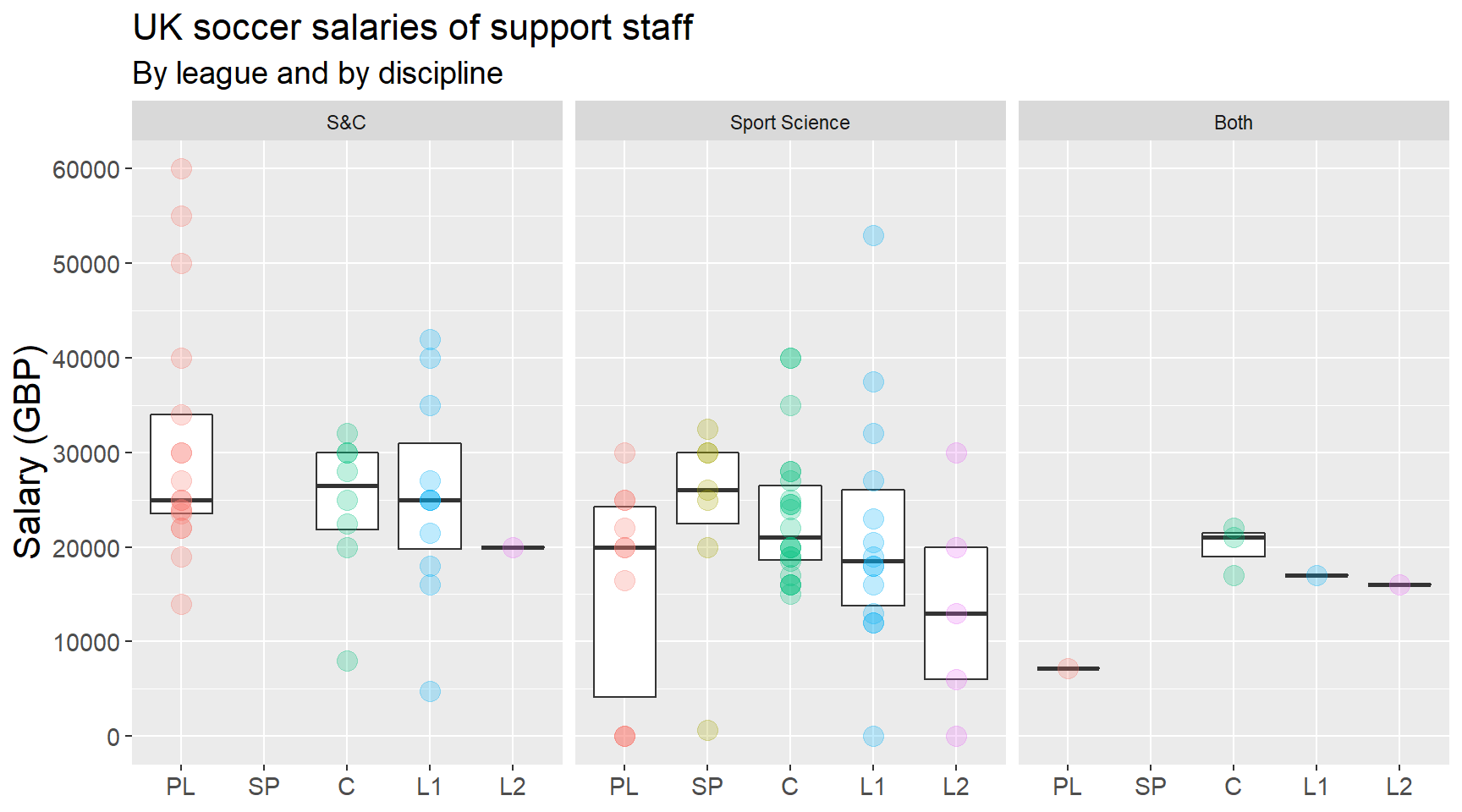
Here is the breakdown of median salaries:
# Calculate median salaries by league and discipline
medianSalariesByLeagueAndDept <- soccerSalariesData3 %>%
    group_by(leagueOfFirstTeam, dept) %>%
    summarise(median = median(salaryGBP, na.rm = TRUE))

# Reorder values by $dept, then by $leagueOfFirstTeam
medianSalariesByLeagueAndDept <- medianSalariesByLeagueAndDept[order(
    medianSalariesByLeagueAndDept$dept, medianSalariesByLeagueAndDept$leagueOfFirstTeam), ]

# Remove duplicate values in $dept for aesthetic purposes
medianSalariesByLeagueAndDept$dept <- c(
    "S&C", rep("", times = 3),
    "Sport Science", rep("", times = 4),
    "Both", rep("", times = 3))

# Rename variables for aesthetic purposes
colnames(medianSalariesByLeagueAndDept) <- c(
    "League in which first team plays", "Discipline", "Median salary (GBP, £)")

# Display the table
medianSalariesByLeagueAndDept %>%
    kable("html") %>%
kable_styling()| League in which first team plays | Discipline | Median salary (GBP, £) |
|---|---|---|
| Premier League | S&C | 25000 |
| Championship | 26500 | |
| League 1 | 25000 | |
| League 2 | 20000 | |
| Premier League | Sport Science | 20000 |
| Scottish Premiership | 26000 | |
| Championship | 21000 | |
| League 1 | 18500 | |
| League 2 | 13000 | |
| Premier League | Both | 7200 |
| Championship | 21000 | |
| League 1 | 17000 | |
| League 2 | 16000 |
Key findings
1. Within-league within-discipline variation is substantial in most cases. Where there is not considerable variation, it is probably due to limited representation within that particular sub-group (e.g., Scottish Premiership sport scientists). Some variation is to be expected, since respondents of different job seniority levels completed the survey. However, the salary variation seen here is in tens of thousands of British Pounds! Seeing this does not breed confidence that a systematic process is used to set performance staff salaries.
In real terms, this means that there are individuals performing similar duties for clubs competing in the same league, but somehow these individuals are being paid wildly different salaries. For instance, three respondents are Lead Academy S&C Coaches for Premier League clubs with salaries of £19,000, £22,000, and £30,000. Similarly, several respondents are Head Academy Sport Scientists for Championship clubs; the lowest salary among them is £27,000 while the highest is £40,000.
Within-league within-discipline variance could be partly accounted for by differences in qualifications, however 80 out of the 102 respondents hold postgraduate degrees (e.g., Postgraduate Certificate, Masters, PhD). It could also represent varying levels of experience or years of service at a particular club, but unfortunately these items were not included in the questionnaire.
2. Within four of the five leagues, S&C coaches are generally paid higher salaries than sport scientists. For League 2, the comparison between disciplines is tenuous because of the small number of responses within each discipline (S&C coaches at League 2 = 1, sport scientists at League 2 = 5). No respondents were S&C coaches working for Scottish Premiership clubs.
3. For S&C coaches and sport scientists, the typical salary for those working in League 1 clubs is not remarkably different to those working for clubs in higher tier leagues (e.g., Premier League, Championship). In part 1 of this series, we plotted salaries by league and by ‘competitive level’ (whether a respondent works for their club’s first team or academy program). This earlier analysis seemed to show a ‘salary gradient’, where typical salaries decreased linearly from higher to lower tier leagues. This pattern is not so clear in this case. However, the true nature of differences or non-differences between leagues would become more apparent with more survey responses, particularly from individuals who fit into the underrepresented sub-groups.
4. A small number of individuals fulfill roles than span both S&C and sport science disciplines. Given that we’re talking about n = 6 here, I’m less focused on the reported salaries as such. What I am interested in is the nature of these dual roles. Is an individual’s workload split between the two disciplines (e.g., 0.5 S&C and 0.5 sport science, or some other proportions)? Are such jobs, in reality, two jobs rolled into one, each of them requiring more than a typical half-time commitment? Or are we just more verbose with our job titles, while retaining the features of jobs from previous eras? Maybe the catch-all ‘Fitness Trainer’ title has simply been replaced by ‘S&C Coach / Sport Scientist’!
Giving consideration to these questions is not just an exercise in discussing semantics (although I do love semantics). Addressing them is crucial for ensuring that individuals in such roles:
- Have sustainable distribution of workloads;
- Are appropriately valued for their specialist knowledge and skills, and possibly wide-ranging responsibilities (e.g., are these individuals considered ‘expert’ in both disciplines, or are they considered to be ‘jacks of all trades’?); and
- Are paid at a level that corresponds with the breadth and depth of their skills, and appreciates the unique challenges faced by those employed in dual roles.
Explore the data on your own
If you’d like to take a look at the data and try your hand at creating / modifying these plots, visit this GitHub repository.
Constructive feedback and comments welcome - get in touch with me via Twitter: @jacquietran.